
# Importar librerias
import pandas as pd # Pandas
import numpy as np # Numpy
import matplotlib.pyplot as plt

from sklearn import preprocessing # para preprocesar los datos
from sklearn import tree # Decision tree
from sklearn.ensemble import AdaBoostClassifier # Ensamble de clasificadores usando AdaBoost
from sklearn.model_selection import cross_val_score # Para realizar crossvalidation
from sklearn.metrics import confusion_matrix, classification_report # Confusion Matrix y reporte de clasificacion
from sklearn.svm import SVC # Clasificador support vector machine
Sonidos
import IPython.display as ipd # Para reproducir audio en el Jupyter Notebook
print('Banana')
ipd.display(ipd.Audio('./Data/Audio/Banana/Track70.wav'))
print('Chair')
ipd.display(ipd.Audio('./Data/Audio/Chair/Track106.wav'))
print('Goodbye')
ipd.display(ipd.Audio('./Data/Audio/Goodbye/Track54.wav'))
print('Hello')
ipd.display(ipd.Audio('./Data/Audio/Hello/Track32.wav'))
print('IceCream')
ipd.display(ipd.Audio('./Data/Audio/IceCream/Track91.wav'))
Banana
Chair
Goodbye
Hello
IceCream
Leer caracteristicas de la señal de audio
Importar las caraceristicas extraidas del audio usando el script audio.R
# Caracteristicas extraidas
train    = pd.read_csv("Data/data-model.csv") # datos de entrenamiento
test     = pd.read_csv("Data/validation.csv") #datos de prueba
train.sample(10) #Tomar aleatoriamente 10 elementos de tabla
| Unnamed: 0 | sound.files | selec | duration | meanfreq | sd | median | Q25 | Q75 | IQR | ... | meanfun | minfun | maxfun | meandom | mindom | maxdom | dfrange | modindx | class | y | |
|---|---|---|---|---|---|---|---|---|---|---|---|---|---|---|---|---|---|---|---|---|---|
| 52 | 70 | Track97.wav | 0 | 1 | 3.963318 | 3.823896 | 2.302780 | 0.963420 | 5.961016 | 4.997596 | ... | 2.739104 | 0.180738 | 8.820000 | 1.195726 | 0.086133 | 8.182617 | 8.096484 | 0.089428 | IceCream | 5 |
| 50 | 68 | Track95.wav | 0 | 1 | 4.588847 | 4.499012 | 2.250706 | 0.610536 | 8.347444 | 7.736908 | ... | 3.256984 | 0.172941 | 14.700000 | 1.815169 | 0.086133 | 11.369531 | 11.283398 | 0.080611 | IceCream | 5 |
| 20 | 27 | Track63.wav | 0 | 1 | 1.869911 | 2.557273 | 1.000404 | 0.546888 | 2.160873 | 1.613985 | ... | 7.441875 | 0.183750 | 14.700000 | 0.823645 | 0.086133 | 1.291992 | 1.205859 | 0.085714 | Goodbye | 2 |
| 32 | 44 | Track83.wav | 0 | 1 | 1.758715 | 2.320001 | 1.251427 | 0.517551 | 1.877141 | 1.359590 | ... | 0.344531 | 0.344531 | 0.344531 | 0.544663 | 0.172266 | 1.550391 | 1.378125 | 0.229167 | Banana | 3 |
| 40 | 58 | Track115.wav | 0 | 1 | 1.613404 | 1.967667 | 1.262465 | 0.619160 | 1.766071 | 1.146911 | ... | 0.445571 | 0.177823 | 1.025581 | 1.306348 | 0.086133 | 5.340234 | 5.254102 | 0.041729 | Chair | 4 |
| 19 | 26 | Track62.wav | 0 | 1 | 1.818739 | 2.435103 | 1.079349 | 0.622763 | 2.086096 | 1.463332 | ... | 14.700000 | 14.700000 | 14.700000 | 0.712553 | 0.086133 | 1.291992 | 1.205859 | 0.089286 | Goodbye | 2 |
| 41 | 59 | Track116.wav | 0 | 1 | 1.607327 | 1.902358 | 1.221825 | 0.573400 | 1.827379 | 1.253979 | ... | 2.602381 | 0.247753 | 14.700000 | 1.109788 | 0.086133 | 5.081836 | 4.995703 | 0.072414 | Chair | 4 |
| 3 | 4 | Track35.wav | 0 | 1 | 1.355439 | 2.126415 | 0.633894 | 0.431348 | 1.246533 | 0.815185 | ... | 13.475000 | 11.025000 | 14.700000 | 0.508594 | 0.086133 | 0.775195 | 0.689063 | 0.137500 | Hello | 1 |
| 38 | 56 | Track113.wav | 0 | 1 | 1.274878 | 1.496729 | 1.142684 | 0.575788 | 1.407235 | 0.831447 | ... | 5.915644 | 0.182231 | 14.700000 | 1.134706 | 0.086133 | 5.254102 | 5.167969 | 0.116667 | Chair | 4 |
| 45 | 63 | Track90.wav | 0 | 1 | 2.082540 | 2.956632 | 1.308302 | 0.382229 | 2.144590 | 1.762360 | ... | 12.250000 | 11.025000 | 14.700000 | 0.375852 | 0.086133 | 1.205859 | 1.119727 | 0.065934 | IceCream | 5 |
10 rows × 27 columns
x = train[["meanfreq","sd","median","Q25","Q75","IQR","skew","kurt","sp.ent","sfm","mode","centroid",
           "peakf","meanfun","minfun","maxfun","meandom","mindom","maxdom","dfrange","modindx"]]
y = train["class"]
Algoritmos de Machine Learning
AdaBoost
# Definir los algoritmos de machine learning
clh = tree.DecisionTreeClassifier(max_depth  = 7)
clf = AdaBoostClassifier(base_estimator= clh,n_estimators=10) # Adaboost
# Entrenar el adaBoost
clf.fit(x,y)
AdaBoostClassifier(algorithm='SAMME.R',
          base_estimator=DecisionTreeClassifier(class_weight=None, criterion='gini', max_depth=7,
            max_features=None, max_leaf_nodes=None,
            min_impurity_decrease=0.0, min_impurity_split=None,
            min_samples_leaf=1, min_samples_split=2,
            min_weight_fraction_leaf=0.0, presort=False, random_state=None,
            splitter='best'),
          learning_rate=1.0, n_estimators=10, random_state=None)
#  Aplicar el modelo a los datos
y_tree_pred = clf.predict(x)
# Valor medio del desempeño con cross validation
print('Desempeño Promedio en el set de entrenamiento = ')
print(np.mean(cross_val_score(clf, x, y, cv=8)))
Desempeño Promedio en el set de entrenamiento =
0.8215277777777779
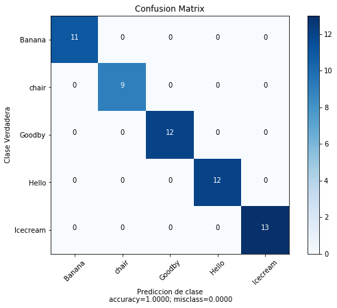
# Ver la matriz de confusion
cm = confusion_matrix(y, y_tree_pred)
print(cm)
[[11  0  0  0  0]
 [ 0  9  0  0  0]
 [ 0  0 12  0  0]
 [ 0  0  0 12  0]
 [ 0  0  0  0 13]]
#Reporte de clasificacion
print(classification_report(y,y_tree_pred))
              precision    recall  f1-score   support

      Banana       1.00      1.00      1.00        11
       Chair       1.00      1.00      1.00         9
     Goodbye       1.00      1.00      1.00        12
       Hello       1.00      1.00      1.00        12
    IceCream       1.00      1.00      1.00        13

   micro avg       1.00      1.00      1.00        57
   macro avg       1.00      1.00      1.00        57
weighted avg       1.00      1.00      1.00        57
test_x = test[["meanfreq","sd","median","Q25","Q75","IQR","skew","kurt","sp.ent","sfm","mode",
               "centroid","peakf","meanfun","minfun","maxfun","meandom","mindom","maxdom","dfrange","modindx"]]
print('Desempeño promedio en el set de pruebas = ')
print(clf.score(test_x,test["class"]))
Desempeño promedio en el set de pruebas =
0.8888888888888888
# función para graficar mejor la matriz de confusion
def plot_confusion_matrix(cm,
                          target_names,
                          title='Confusion matrix',
                          cmap=None,
                          normalize=True):
    """
    given a sklearn confusion matrix (cm), make a nice plot

    Arguments
    ---------
    cm:           confusion matrix from sklearn.metrics.confusion_matrix

    target_names: given classification classes such as [0, 1, 2]
                  the class names, for example: ['high', 'medium', 'low']

    title:        the text to display at the top of the matrix

    cmap:         the gradient of the values displayed from matplotlib.pyplot.cm
                  see http://matplotlib.org/examples/color/colormaps_reference.html
                  plt.get_cmap('jet') or plt.cm.Blues

    normalize:    If False, plot the raw numbers
                  If True, plot the proportions

    Usage
    -----
    plot_confusion_matrix(cm           = cm,                  # confusion matrix created by
                                                              # sklearn.metrics.confusion_matrix
                          normalize    = True,                # show proportions
                          target_names = y_labels_vals,       # list of names of the classes
                          title        = best_estimator_name) # title of graph

    Citiation
    ---------
    http://scikit-learn.org/stable/auto_examples/model_selection/plot_confusion_matrix.html

    """
    import matplotlib.pyplot as plt
    import numpy as np
    import itertools

    accuracy = np.trace(cm) / float(np.sum(cm))
    misclass = 1 - accuracy

    if cmap is None:
        cmap = plt.get_cmap('Blues')

    plt.figure(figsize=(8, 6))
    plt.imshow(cm, interpolation='nearest', cmap=cmap)
    plt.title(title)
    plt.colorbar()

    if target_names is not None:
        tick_marks = np.arange(len(target_names))
        plt.xticks(tick_marks, target_names, rotation=45)
        plt.yticks(tick_marks, target_names)

    if normalize:
        cm = cm.astype('float') / cm.sum(axis=1)[:, np.newaxis]


    thresh = cm.max() / 1.5 if normalize else cm.max() / 2
    for i, j in itertools.product(range(cm.shape[0]), range(cm.shape[1])):
        if normalize:
            plt.text(j, i, "{:0.4f}".format(cm[i, j]),
                     horizontalalignment="center",
                     color="white" if cm[i, j] > thresh else "black")
        else:
            plt.text(j, i, "{:,}".format(cm[i, j]),
                     horizontalalignment="center",
                     color="white" if cm[i, j] > thresh else "black")


    plt.tight_layout()
    plt.ylabel('Clase Verdadera')
    plt.xlabel('Prediccion de clase\n accuracy={:0.4f}; misclass={:0.4f}'.format(accuracy, misclass))
    plt.show()
plot_confusion_matrix(cm           = cm,
                      normalize    = False,
                      target_names = ['Banana', 'chair', 'Goodby', 'Hello','Icecream'],
                      title        = "Confusion Matrix")
Support Vector Classification (SVC)
# Configurar el clasificador SVC
svcfit = SVC(C=0.01, kernel='linear')
x =  preprocessing.scale(x) # Escalar los datos
# Entrenar el modelo
svcfit.fit(x, y)
SVC(C=0.01, cache_size=200, class_weight=None, coef0=0.0,
  decision_function_shape='ovr', degree=3, gamma='auto_deprecated',
  kernel='linear', max_iter=-1, probability=False, random_state=None,
  shrinking=True, tol=0.001, verbose=False)
# Predicion con el modelo
y_svc_pred =svcfit.predict(x)
# Valor medio del desempeño con cross validation
print('Desempeño Promedio en el set de entrenamiento = ')
print(np.mean(cross_val_score(svcfit, x, y, cv=8)))
Desempeño Promedio en el set de entrenamiento =
0.6329861111111111
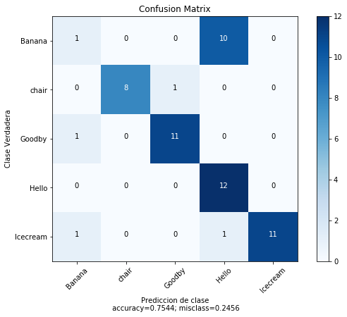
# Matriz de confusion
cm = confusion_matrix(y,y_svc_pred)
print(cm)
[[ 1  0  0 10  0]
 [ 0  8  1  0  0]
 [ 1  0 11  0  0]
 [ 0  0  0 12  0]
 [ 1  0  0  1 11]]
#Reporte de clasificacion
print(classification_report(y,y_svc_pred))
              precision    recall  f1-score   support

      Banana       0.33      0.09      0.14        11
       Chair       1.00      0.89      0.94         9
     Goodbye       0.92      0.92      0.92        12
       Hello       0.52      1.00      0.69        12
    IceCream       1.00      0.85      0.92        13

   micro avg       0.75      0.75      0.75        57
   macro avg       0.75      0.75      0.72        57
weighted avg       0.75      0.75      0.72        57
test_x     =  preprocessing.scale(test_x)
print('Desempeño Promedio en el set de test = ')
print(svcfit.score(test_x,test["class"]))
Desempeño Promedio en el set de test =
0.7777777777777778
plot_confusion_matrix(cm           = cm,
                      normalize    = False,
                      target_names = ['Banana', 'chair', 'Goodby', 'Hello','Icecream'],
                      title        = "Confusion Matrix")
Phd. Jose R. Zapata